MFB2 Temperature anisotropy

16/02/2026 - 27/02/2026

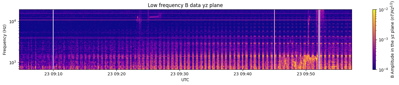
We analyze the time period during the wave signature measured by the PWI search coil magnetometer spanning 23/06/2022 9:45 to 9:51 denoted with the pink lines.
Pasted image 20260218211745.png

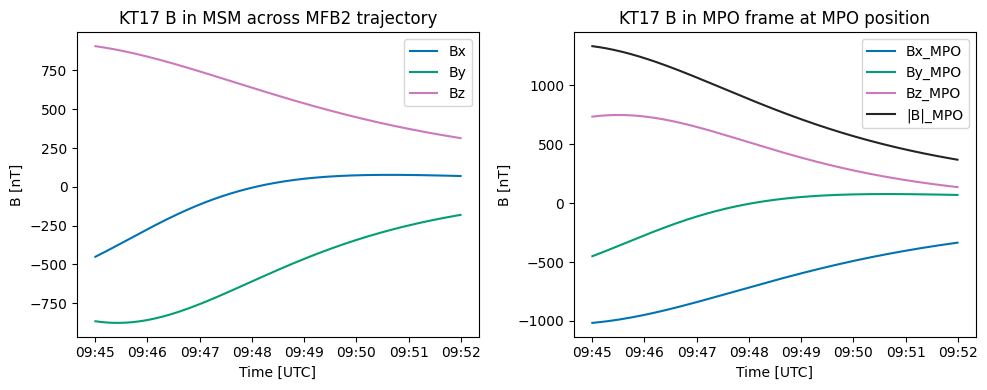
The trajectory of the spacecraft at the time is shown below in the MagnetoSpheric Mercury (MSM) Frame.

We can get the magnetic field and its direction across this trajectory through the KT17 Model in the MagnetoSpheric Mercury (MSM) Frame and transform it in the MPO frame using SPICE kernels.

Pasted image 20260310161808.png

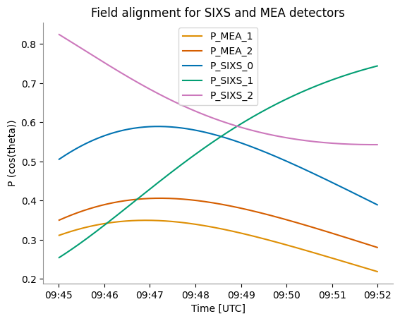
We can also get the direction of the P0,P1,P2 SIXS detectors in the MPO frame by transforming a $z = (0, 0, 1)$ vector from 'MPO_SIXS-P-0' frame to 'MPO_SPACECRAFT'. By taking the vector product with the direction of the magnetic field we can compute the pitch angle $θ$ :

\cos θ = \frac{\vec{a} \cdot \vec{b}}{| \vec{a} | | \vec{b} |}

Here we plot the differential flux of the high energy electrons during the whistler signature in one axes, and the calculated pitch angle of the detector on the other.

To keep the same scale we can plot it in one figure, where green refers to the P0 detector, blue to P1 and red to P2.

We can notice some relative flux difference in the measurement of each viewing direction, however small since the detectors happen to be in quasi-oblique angles. Assuming a simple temperature anisotropic distribution function, we can derive a measure of the parallel and perpandicular flux anisotropy by comparing these relative flux measurements.

Below two simple temperature anisotropic maxwellians are shown in the velocity space, parallel and perpandicular to the magnetic field:

f (v, θ) d^{3} ν = \frac{n}{T_{⊥} T_{∥}^{1 / 2}} {(\frac{m}{2 π k_{B}})}^{\frac{3}{2}} \exp (- \frac{m v_{⊥}^{2}}{2 k_{B} T_{⊥}} - \frac{m v_{∥}}{2 k_{B} T_{∥}}) d^{3} ν

= \frac{n}{T_{⊥} T_{∥}^{1 / 2}} {(\frac{m}{2 π k_{B}})}^{\frac{3}{2}} \exp (- \frac{m v^{2} \sin^{2} θ}{2 k_{B} T_{⊥}} - \frac{m v^{2} \cos^{2} θ}{2 k_{B} T_{∥}}) d^{3} ν

In one case the parallel temperature is double the perpandicular and vise-versa. The two cones depict the looking directions of P0 and P1 detector of SIXS while the grey area highlights the energy range that they will sample. The P0 detector has similar looking direction with the MEA instruments during the cruise phase. The pink highlighted area depicts the energy range that the MEA will sample. The angles denoted with blue are the pitch angles of each detector.

[ ] cahnge angles
In these cases, the calculated energy flux that the three SIXS detectors would measure in one timestep (for a particular set of pitch angles $θ_{1}, θ_{2}, θ_{3}$ ) can be computed by integrating over a fixed solid angle in Spherical coordinates (if the $v^{2}$ dependancy is not clear you can find a more detailed explanation here: Maxwell - Boltzmann Distribution):

F = \int f (u, θ) v^{2} d v d Ω \propto \frac{n}{T_{⊥} T_{∥}^{1 / 2}} {(\frac{m}{2 π k_{B}})}^{\frac{3}{2}} \exp (- \frac{m v^{2} \sin^{2} θ}{2 k_{B} T_{⊥}} - \frac{m v^{2} \cos^{2} θ}{2 k_{B} T_{∥}}) * v^{2}

For one timestep and the three different pitch angles of SIXS we would get the following Boltzmann distributions, if we could sample all the energies:

change title
Although angularly sparsely sampled, we can derive information about the initial anisotropy by computing the weighted sum of the projection of the fluxes parallel and perpendicular to the magnetic field. The units here are set arbitrarily since we are not interested in the actual temperature but on how well we could characterise a flux anisotropy with this metric.

F_{∥} = \frac{\sum_{θ_{i}} \cos^{2} θ_{i} \sum_{ν} F_{θ_{i}} (ν)}{\sum_{θ_{i}} \cos^{2} θ_{i}}

F_{⊥} = \frac{\sum_{θ_{i}} \sin^{2} θ_{i} \sum_{ν} F_{θ_{i}} (ν)}{\sum_{θ_{i}} \sin^{2} θ_{i}}

A bounded measure of the anisotropy $\in [- 1, 1]$ where -1 is fully perpendicular, +1 is fully parallel and 0 is isotropic can be derived through:

A_{s y n t h} = \frac{F_{∥} - F_{⊥}}{F_{∥} + F_{⊥}}

where $A > 0$ means

F_{∥} > F_{⊥}

and $A < 0$ means

F_{⊥} > F_{∥}

For the pitch angles that correspond to the whistler signature and the synthetic distribution we get:

The 0 value is in line with the fact that the three pitch angles reach very similar values around 9:49. The sign of A is in line with the synthetic temperature anisotropy. This means that this is a suitable measure for a sparse indication about the perpandicular and parallel flux anisotropy, given a simple temperature anisotropic distribution

This hypothesis of a monotonically anisotropic shape of the distribution function is a strong one, and therefore this metric would give us limited information when sampling a more complex distribution. We can further investigate the case of the non-monotonically changing function by sampling the simulated distribution function of the PIC code, where this seems to be the case. From the full VDF we keep the particles that are inside FOV of each detector for each timestep. Since we are interested only on the pitch angle dependence we can keep all the particles that have the pitch angle of the detector with a $\pm \frac{F O V}{2}$ margin to increase our statistics. We then keep the particles that have speed directed towards the detector, assuming the active area is a disk of arbitrary radius R. For one timestep and one detector, this is spatially depicted below:

We can see the same picture in velocity space where each plot is a different slice of the parallel - perpendicular plane relative to the magnetic field. The cones indicate the viewing directions of P_0, P_1 and P_2 and the gray areas their energy range. We see that although we have a mostly parallel anisotropic function, there is more heating in particular oblique direction, which in particular looking direction - when sampled - will give a negative A.

The time series of the computed energy flux for each detector is shown below. From this we can again calculate the anisotropy index A for the simulated VDF and the detector pitch angles. We see variations from positive to negative A depending on the detector pitch angles.

mean velocity introduces anisotropy

The actual SIXS measurements are in the units of energy flux and therefore our calculations will take the following form:

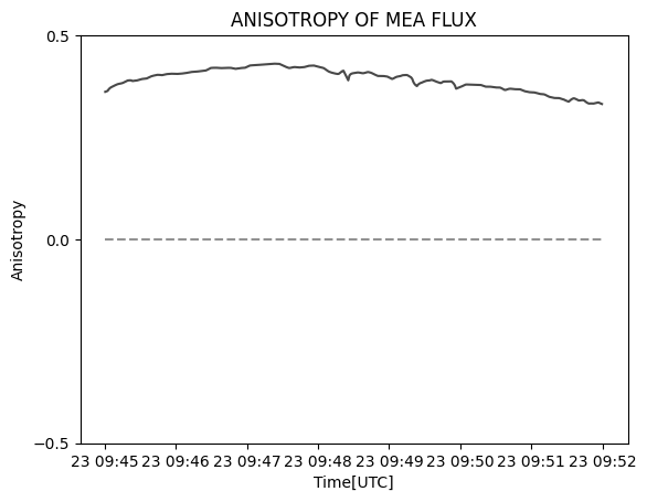
F_{∥} \propto \frac{\sum_{E, θ} \cos^{2} θ \cdot F_{E} (θ, E)}{\sum_{θ} \cos^{2} θ}

F_{⊥} \propto \frac{\sum_{E, θ} (1 - \cos^{2} θ) F_{E} (θ, E)}{\sum_{θ} 1 - \cos^{2} θ}

Applying the anisotropy metric to the data returns:

A = \frac{F_{∥} - F_{⊥}}{F_{∥} + F_{⊥}}

The change of sign in the actual data could indicate either a non-monotonically anistoropic distribution (ex butterfly shape) , or a change on the nature of the interaction between the wave and the particles. The test on the simulated distribution function is a good example of the first case, where the VDF was static, however the angles of the detectors allowed for sampling of different features.

The Mercury Electron Analyser (MEA) available channels during cruise phase sample both very similar directions.
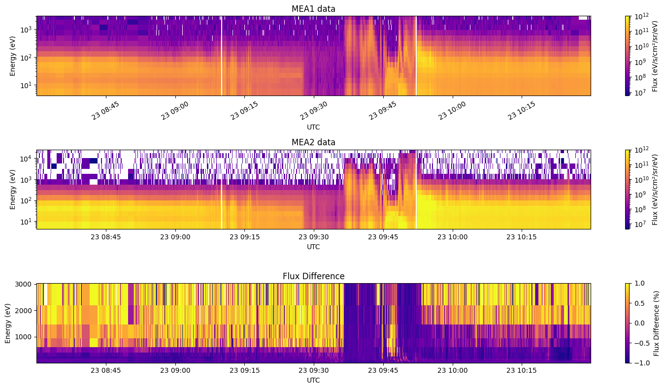
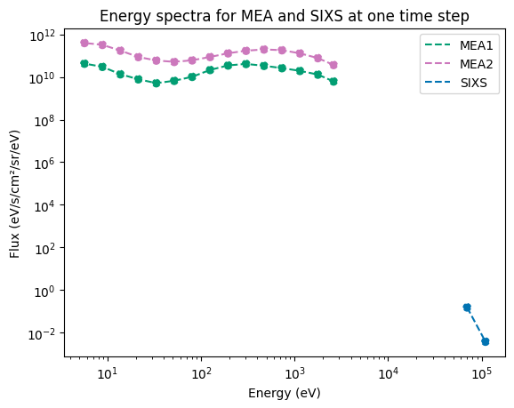
Pasted image 20260312133529.png|697

Comparison between SIXS and MEA cannot be performed, unless we have a good way of estimating the distribution function given only the 2 tail energy points of the SIXS measuremnts:

Pasted image 20260312133559.png|372

The angular separation of the detectors is small and therefore it is difficult to differentiate anisotropy due to pitch angle difference versus anisotropy due to sensitivity of each instrument and particular configuration during cruise phase.If we were to compute the flux anisotropy, we would get a mostly parallel anisotropy. We cannot trust the absolute value but we could possibly take into account the trend (ascending, descinding)
Pasted image 20260312133816.png|330 Pasted image 20260312134025.png|342

exclude secondary electrons (30eV)
[ ]