Python implementation in git open source repository

Hough: Finds lines
Duda: [[Duda - Hough Transform.pdf]] - Finds lines and curves
Farber: [[Farber - Hough Transform.pdf]] - Any given curve
Python implementation: [[HoughT.pdf]] - Any shape

Hough Transform for lines

Video explanation of Hough transform: https://www.youtube.com/watch?v=XRBc_xkZREg

The point where all the lines in parameter space intersect, describe the parameters of the line we are looking for in the image space.

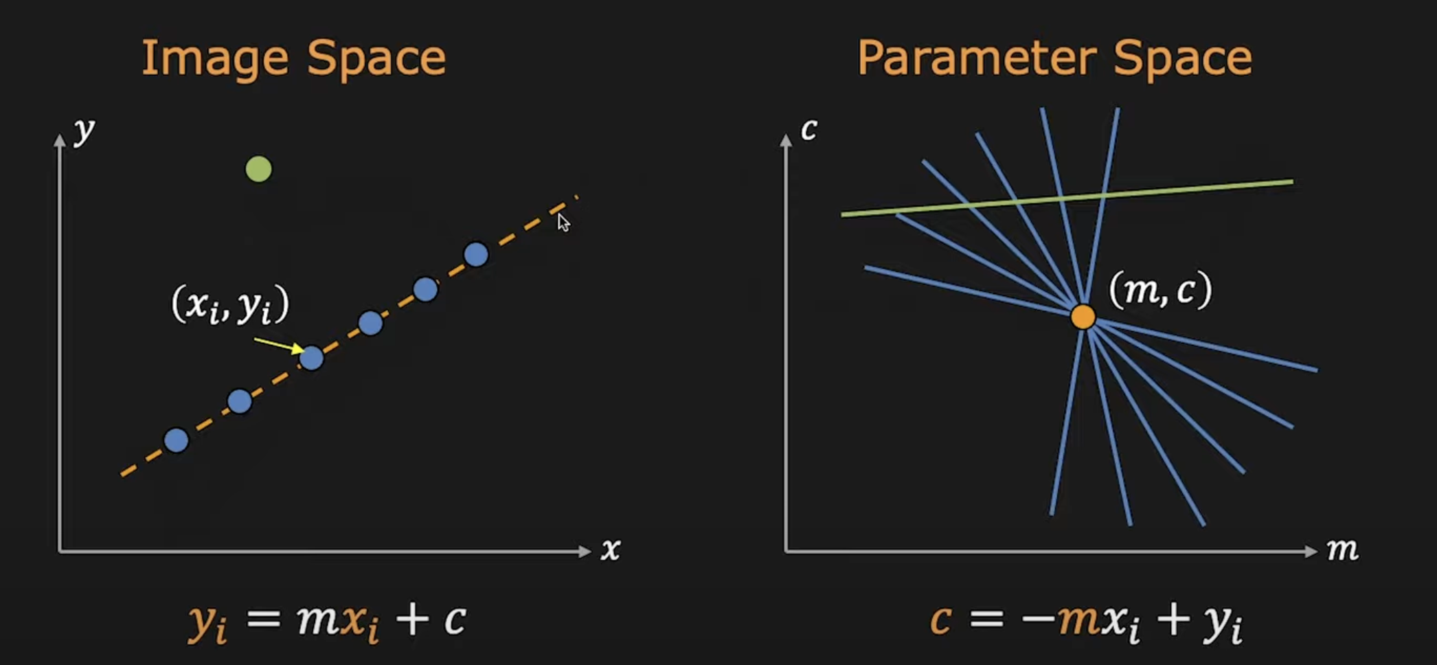
1. Quantize parameter space in a accumulator array
2. Set all the cells to zero A(m,c) = 0
3. For each image space point x,y we increment all the point of the array that the m,c line passes through: $A(m,c)=A(m,c)+1$ for $c=-m{x}_i+y_i$
4. The largest cell value is the point of intersection --> coordinates are the parameters of line in image space

-- We dont use cartesian because the slope m can go to infinity => overflow
-- We use instead polar parameterisation , θ , ρ = finite

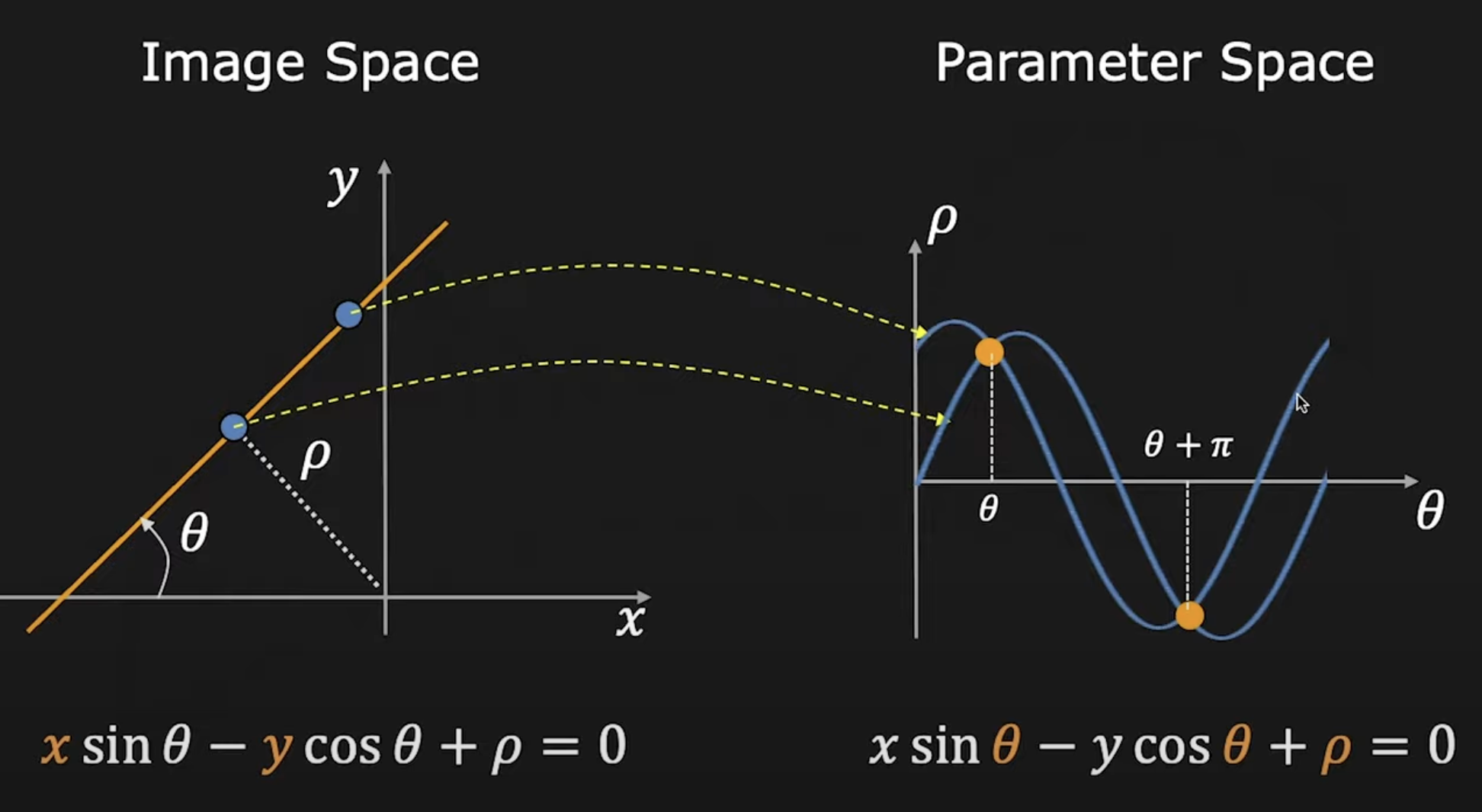
-- Bin pixels before transforming to reduce noise

Circle detection

The parameter space of a circle is itself a circle.

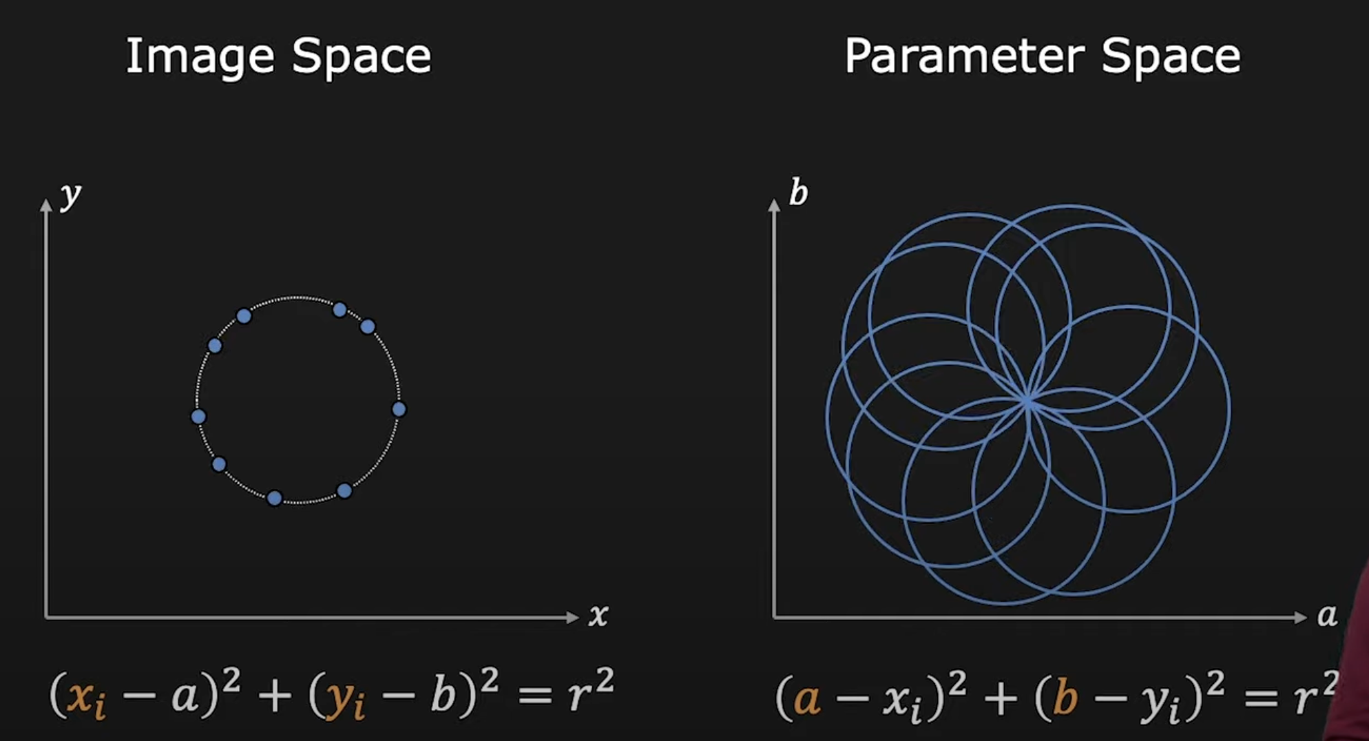
If we dont know the radius, we got to a 3D parameter space and for each point we vote for a cone.

Generalized Hough transform

Hough-like method or custom curve voting scheme

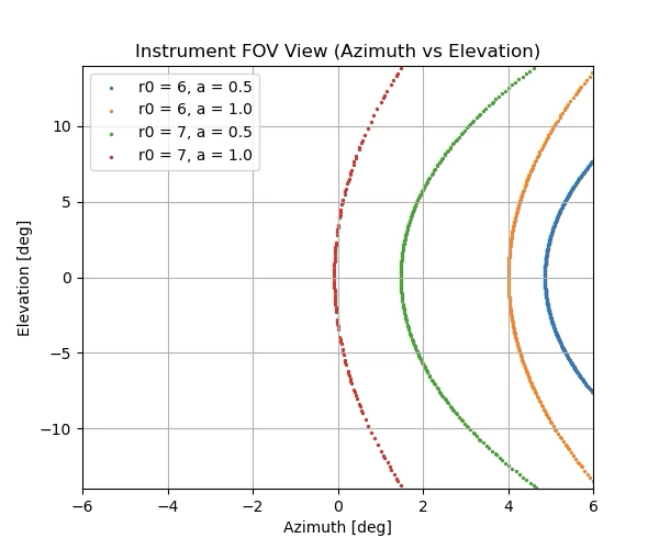
We adopt a Hough-like voting approach by projecting candidate curve templates into the instrument’s field of view and accumulating pixel intensities along each curve to determine the best match.

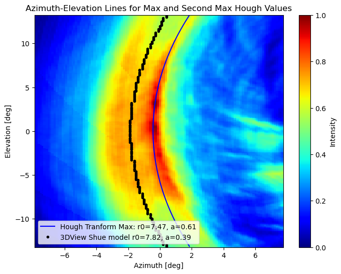
For a set of initial parameters of the magnetopause model in use, we compute the tangent points as in Numerical Solution & Performance. By applying the Coordinate transformation from GSE to SXI we get a set of discretized curves. We interpolate the curves inside the FOV and rasterize them to the pixel grid of the image.
!x!300
For each parameter set we can plot the intensity of the image in its cross-section with the curve:

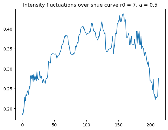
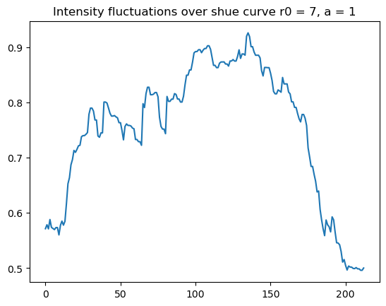
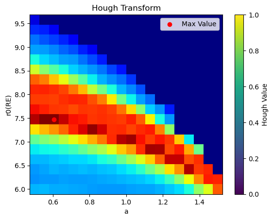
We compute a large set of curves with different a and r0:

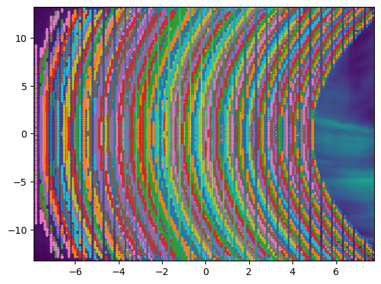
We create a table with the mean intensity over each curve for each set of parameters. This can be plotted in the parameter space as a table, while its maximum value is plotted on the image space as a curve.