Arc detection problems

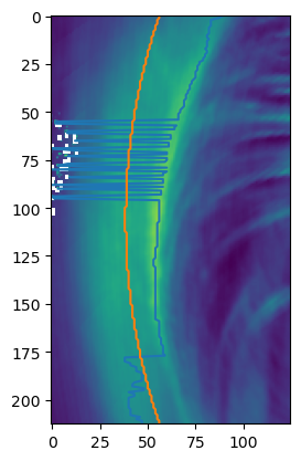
1. When tracing the maximum intensity arc there are jumps to the second maximum, especially in the edges Cube and Image tests
   Local maxima and minima:
   
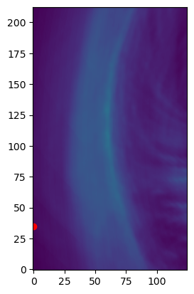
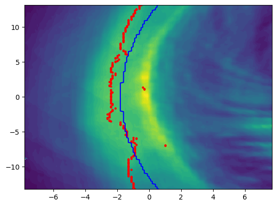
2. When trying to extract separately the images without the Shue mask, there are some simulation discontinuities that peak the value of specific pixels to the gods Correlation of Intensity to tangent direction

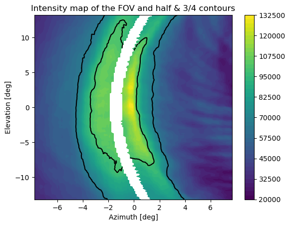
Image with Shue model mask.	Image without shue model mask.	Fixed image
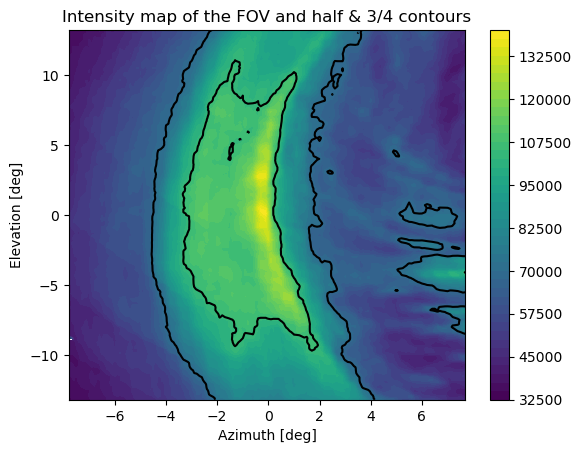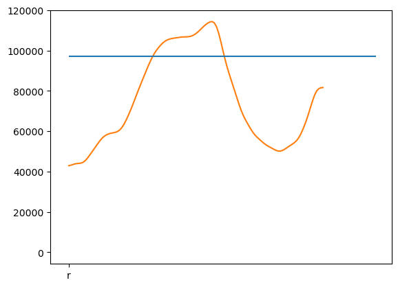
Contours indicate the 0.5 and 0.75 intensity thresholds	The red dot is the pixel that peaks the values.	Find the values above a threshold and set them to None.

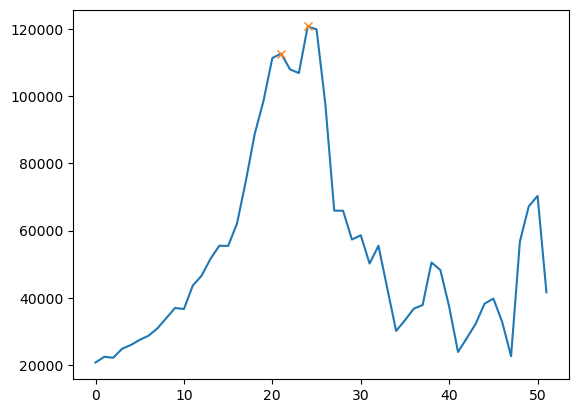
The threshold effectively discards the discontinuities, but problems arise for single pixel peaks when detecting the maximum intensity.Here the low value discontinuities have still a significant value and are recognized as the maximum of the row.

Two discontinuity problems remain: jumps between arcs, and jumps to simulation errors.

3. When trying to extract the 2nd maxima with scipy, the method fails for several rows depending on the image. Here the 2nd maxima detected after applying 2σ gaussian smoothing to each row is shown. Maximum of the second gradient could possibly work better for these rows (row example - 2nd image)
   

Discontinuity solutions

1. Discard jump values by detecting large azimuth differences between steps

 if D_azimuth>2degrees:
	discard
	if d_azimuth<1degrees:
	discard
	else
	take into acount

2. Hough Tranform : Define the curve that we are trying to detect -> returns an array with all the detected curves in the image. The first ones are the most prominent ones.
   -- For the minimum, restrain the range between the two maxima and find minimum.

The second approach is more robust and is a standard computer vision algorithm

Solution

Testing a polynomial hough approach

When trying to fit a 2nd polynomial, we have 3 degrees of freedom and therefore a 3 dimensional parameter space.

This is relatively fast but cannot take into account the asymmetry of the true arc (left). If we introduce a $y^3$ term this anisotropy can theoretically be fitted, although in practice the 3rd order term blows up, and the resulting curve rarely converges (even with very small initial coefficients given).

Shortly, it is evident that not only is it a slow solution and without a measure of the error - but it is also difficult to implement while ensuring convergence and not overfitting.

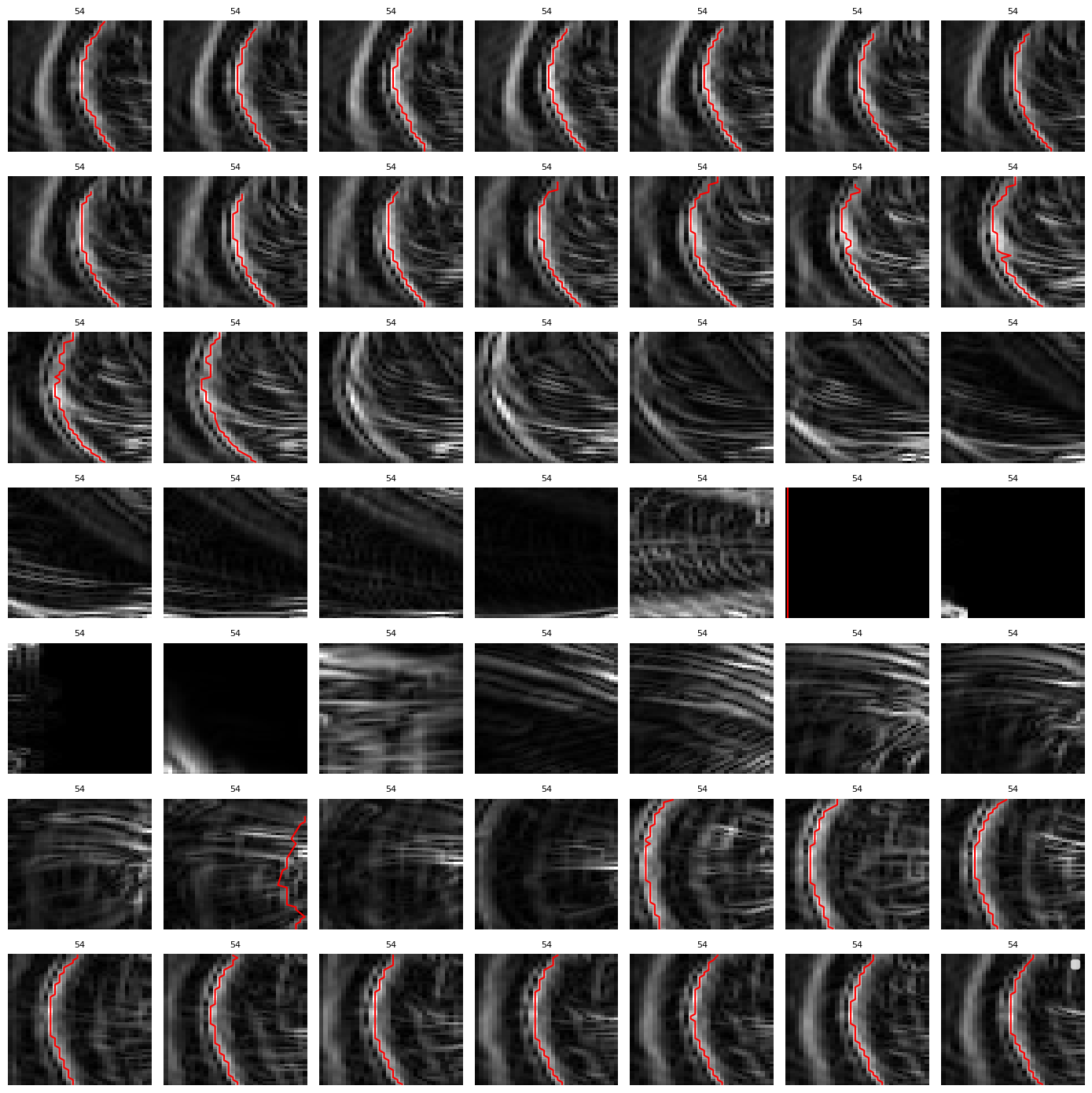
Filters and maximum extraction approach

Thus we move back to the maximum extraction for each line approach, where we need to discard the noise that cause the jumps.

Here we pass the images through a edge detection filter skimage.filters.sobel. We then find the maximum azimuth index for each elevation and discard the ones that have a jump larger than 2 indexes. In the pictures approaching the magnetopause random arcs are being detected, so we discard the filtered array that are smaller than 20 points (the rest have been discarded due to jumps), as well as the ones that have an overage intensity smaller than 0.2 normalized. The result is: