Model magnetopause construction
Model magnetopause projection
20-21/02/25
In order to verify the position of the simulated magnetopause in the pictures (the shue model with the correct parameters is not a good fit) we need to extract the 3D surface from the 3Dcubes and project it in our FOV.
1st approximation method - Principle: There is not x-ray emission inside the magnetosphere :
-
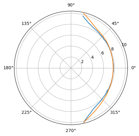
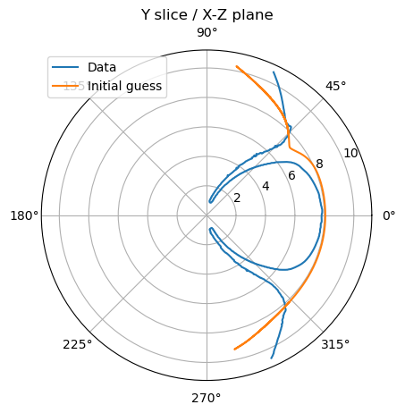
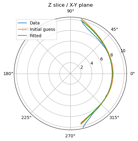
Find 0 (1E-6) emissivity contours for z and y slices
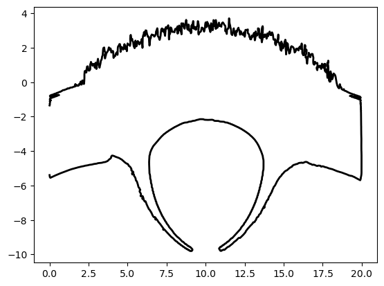
-
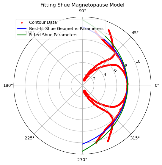
Convert them into polar and combine in one array. We will not take into account asymmetries so we will fit for both directions at the same time. We fit the shue model and get the
and for the best fit (blue line) -
We define a function to minimize with scipy to approximate the corresponfing bz, vx and n / Dp of the shue model parameters. We find: Bz = 10nT, vx = 800km/s and Dp = 12.29 (green line)
-
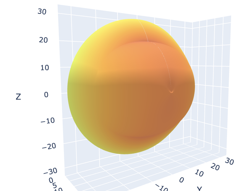
Insert these parameters into 3D view and recompute the shue model surface. Resulting model projection:
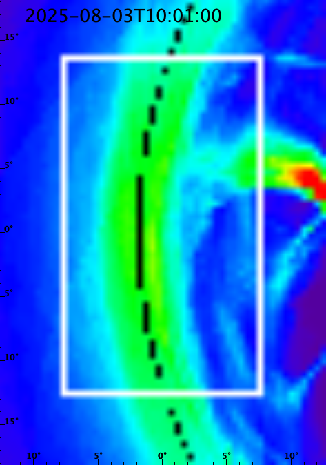
This indicated that the magnetopause may be indeed on the brightest arc or close to it. A better model of the MHD magnetopause needs to be inserted to know with percision.
Fitting the Lin model
24-28/02/25
The fit of the Shue model is not sufficient to confidently correlate the maximum emissivity with the magnetopause position (the fit is not reliable). At the same time the black line seems to be in the region between the two intensity peaks (a bit outside the maximum intensity) while the fit also overestimates the radius for many angles. This is a good indication that we need a better description of the magnetopause to accurately characterize the correlation.
We can do that by fitting the Lin model to the two slices, computing the 3D surface, and project it according to the attitude of the satellite. While trying to fit the Lin model several problem arose:
- The Lin Model#General expression of the Lin model seems to have 18 independent variables. A fit can be performed but it usually results in local minima. This could potentially be fixed by using better fitting techniques (ex. MCMC). For this test I used the Nelder and Mead method (same as CMEM).
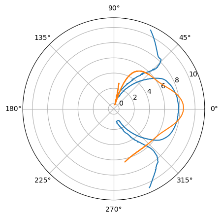
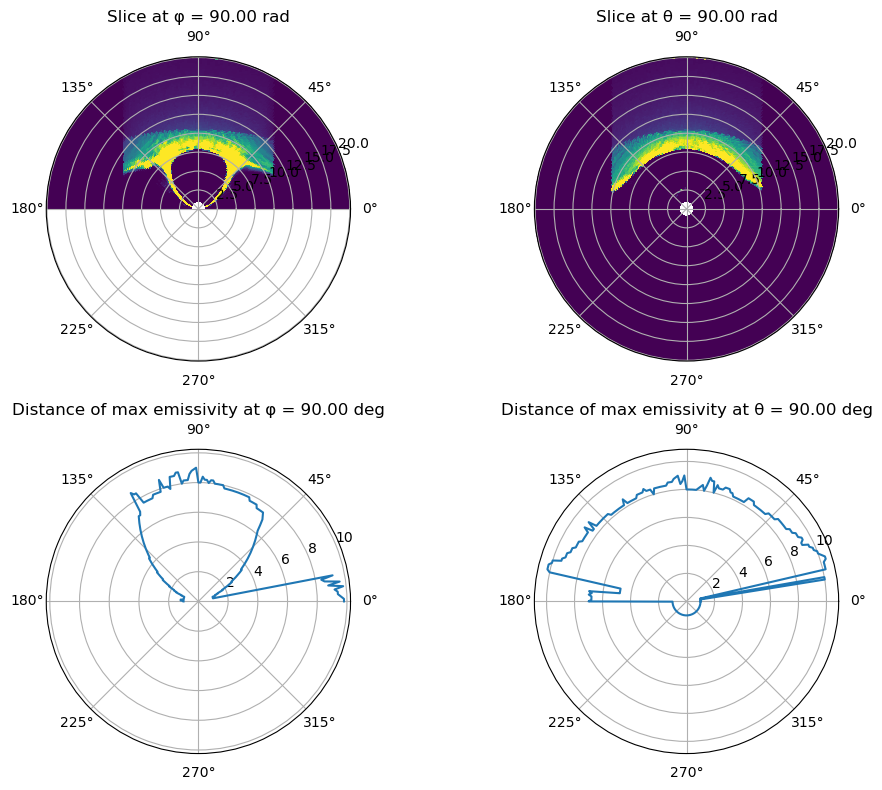
We can see that the z slice can be fitted quite accurately but it has difficulty fitting the y slice - cusps - When computing the parametrized model
discontinuities arise for particular phi angles, and the response for theta = 0 is unpredictable. The phi dependence is completely inaccurate.(typo in the formula of the code). The surface for the simulation conditions (Pd,Pm,Bz,tilt) is already a better fit that the Shue model. The Nelder-Mead fit with a simple loss function, degrades the fit.
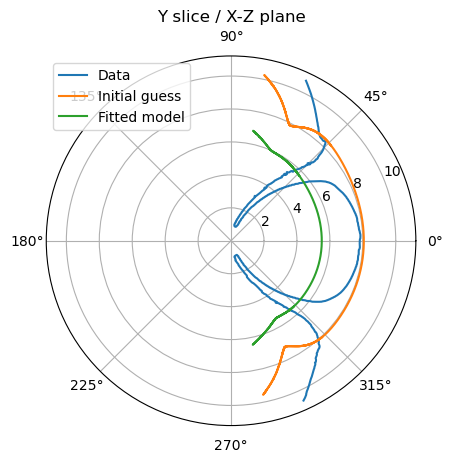
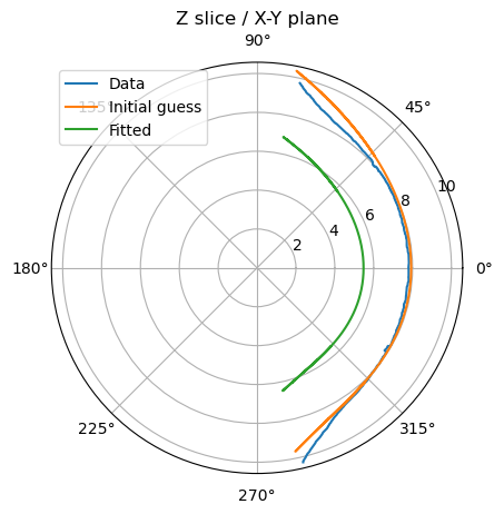
That is caused by the larger dips in the y slice compared to the model. When fitting only the z-slice we have a better response :
When trying the Lin Model#CMEM model good initial guess is still necessary and the radius is still underestimated due to the cusps.
Extracting the surface from the model
Using the definitions provided in Andrew Read's paper and the code provided by here. The resulting cuts of the emissivity cubes for
To project this into the images and compare with the maximum intensity detected, we need to modify the Coordinate transformation from GSE to SXI function to work for a random numerical surface.
g]]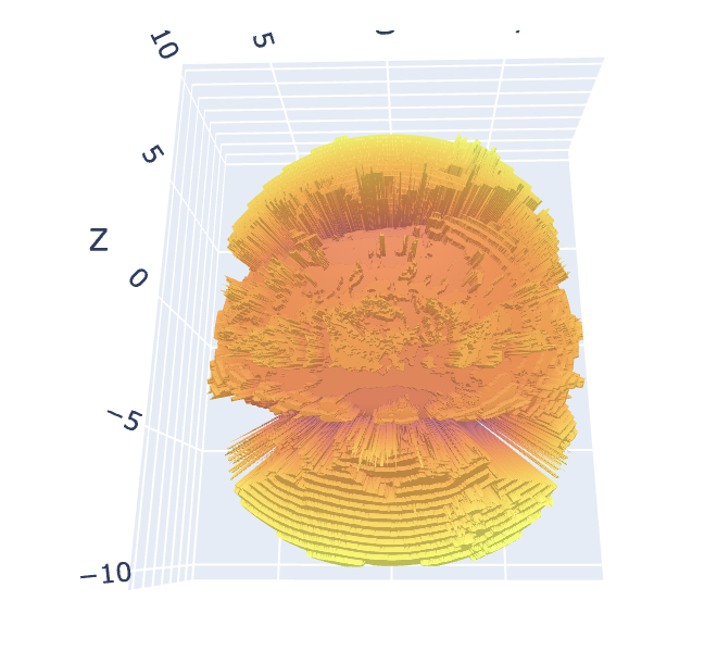
People need to seriously learn how to not do typos in their math formulas.
Liu model: