Numerical Solution & Performance
For a set of 50 images the code initially needed 50 min to run. By improving the interpolation it now running in 25 min. Significant improvements are still needed (solver, sampling, fitting).
It seems I was fitting ✨nonsense✨
The glob.glob() function return the images in random order - I was correlating random viewing directions to random images (same for Correlation of Intensity to tangent direction)
Current performance: 5min for 50 images
The correlation of the outputed parameters with the time and orbit can be found in Benchmarking
Problems
Depending on the image geometry several problems arise:
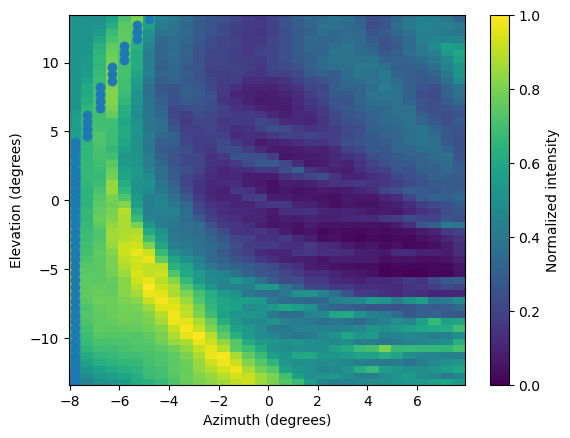
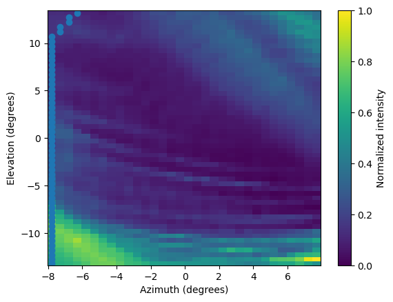
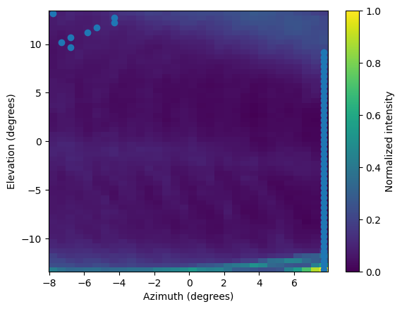
-- Clipping - Interpolator: When the model starts to leave outside the FOV the interpolator clips the values to the edge of the image.
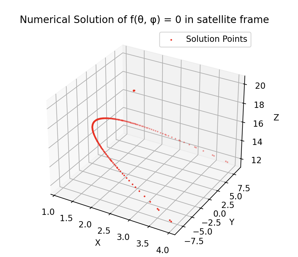
-- Inside the magnetopause - Solver: as soon as we enter the magnetopause, the outputted curve displays discrepancies. In other cases random points are being returned that do not resemble a curve. This is because the solution has less than 5 point (4 needed for the cubic interpolation) and the interpolator returns None for the az , el indexes. The r0 that is return is just the first argument of the initial fitting array - in this case 6 RE.
-- Empty xml file - 3DView: in index 26, 3DView outputs an empty image
Solutions
Interpolation
Initial interpolator was too slow, mainly beacuse:
- I was flattening the array and doing the interpolation separately for az end el having to sample multiple times the same pixels just to make sure that there will be no gaps in elevation ==> interp1D(elevation,azimuth) directly for all the el_image values
- Instead of transforming from el,az coordinate space to index space directly I was searching the values inside the array
Performance: 0.06sec ==> 0.0007sec (2 orders of magnitude faster)
Sampling
In order to check
Solver
Having calculated analytically the equation that returns the Tangent points to SXI in GSE we can turn this into a numerical function using lamdify and solve numericaly for φ and θ:
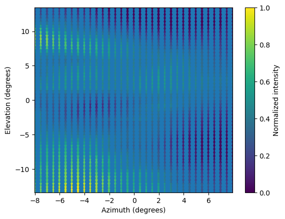
Apply mask to values lower than an arbitrary threshold